Math 202C – Page 3 – Jonathan Novak

Math 202C: Lecture 3

*** All problems in this lecture due April 12 at 23:59 ***

We return to the general setting of a finite, connected, simple graph $G=\mathrm{Cay}(S,T)$ , and as before $\mathcal{C}(S)$ the Hilbert space with orthonormal basis $|\pi\rangle, |\rho\rangle,|\sigma\rangle,\dots$ . In Lecture 1 we introduced the metrics level set linear operators $L_0,L_1,L_2,\dots$ in $\mathrm{End}\mathcal{C}(S)$ which act on vertices according to

$L_r|\rho\rangle = \sum\limits_{\substack{\sigma \in S \\ \mathrm{d}(\rho,\sigma)=r}} |\sigma\rangle.$

We argued the case that these operators are quite fundamental: $L_0=I$ is the identity operator, $L_1=K$ is the adjacency operator,

$D = \sum\limits_{r=0}^\infty rL_r$

is the distance operator,

$\Omega_q=\sum\limits_{r=0}^\infty q^r L_r$

is the exponential distance operator. However, the selfadjoint operators $L_0,L_1,L_2,\dots$ and the subalgebra of $\mathrm{End}\mathcal{C}(S)$ they generate are not easy to understand.

Problem 3.1. Show that $\langle \sigma|L_sL_r|\rho\rangle$ is the cardinality of the intersection of the sphere of radius $r$ centered at $\rho$ with the sphere of radius $s$ centered at $\sigma$ .

So, the matrix elements of the commutator

$[L_s,L_r]=L_sL_r - L_rL_s$

are differences of intersection numbers,

and if it seems difficult to characterize graphs for which all such differences are zero, that’s because it is. There is one much-studied class of graphs which does have the property that metric level set operators $L_0,L_1,L_2,\dots$ commute.

Problem 3.2. Show that if $G$ is a distance regular graph, then $[L_r,L_s]=0.$

The following is the only restricted situation in which I personally know a simple combinatorial characterization of commutativity of the metric level set operators (it is likely that an actual graph theorist would know more).

Problem 3.3. Suppose $G$ has diameter $2.$ Prove that the metric level set operators on $G$ commute if and only if $G$ is a regular graph. (Hint: the basic reason behind this is that in a graph of diameter $2,$ the metric does not contain any more information than the adjacency relation).

I am torturing you (us, really) with these combinatorial considerations because I want to further hammer home the point that Cayley graphs are much easier to understand than general graphs due to the underlying group structure, which is reflected in the behavior of linear operators acting on the vertices of the graph.

Suppose that $S=\{\pi,\rho,\sigma,\dots\}$ is a finite group, so that $\mathcal{C}(S)$ is the convolution algebra of this group. For any arbitrary subset $A \subseteq S,$ we write

$|A\rangle=\sum\limits_{\pi \in A}|\pi\rangle,$

which is simply the indicator function of the set $A$ . It is a very convenient abuse of notation to also simply write $A$ for the image of $|A\rangle$ in the right regular representation, i.e. we identity the set $A \subseteq S$ with the operator $A \in \mathrm{End}\mathcal{C}(S)$ defined by

$A|\rho\rangle = |\rho\rangle|A\rangle=\sum\limits_{\pi \in A} |\rho\pi\rangle.$

Recall from Math 202B that we have a tracial state

$\langle \cdot \rangle \colon \mathcal{C}(S) \longrightarrow \mathbb{C}$

on the convolution algebra of $S$ defined by

$\langle A \rangle := \langle \iota |A\rangle,$

where $\iota \in S$ is the group identity. In other words, $\langle A \rangle$ is the coefficient of the vector $|A\rangle$ in the group basis $|\pi\rangle,$ which is the same thing as the value of the function $A$ at the point $\pi=\iota.$ Here is a second under-appreciated characterization of this important functional, which is often referred to as the canonical group trace.

Problem 3.4. Prove that all diagonal matrix elements $\langle \pi | A |\pi\rangle$ of the image $A \in \mathrm{End}\mathcal{C}(S)$ of $|A\rangle\in \mathcal{C}(S)$ in the regular representation are equal to the same number, and that that number is $\langle A \rangle.$ Hence conclude (as was already shown in Math 202B) that the $\langle A \rangle =\frac{1}{|S|}\mathrm{Tr} A.$

Now to Cayley graphs. We continue with a finite group $S$ and select inside it a symmetric set of generators $T$ , giving us the Cayley graph $G = \mathrm{Cay}(S,T).$ As discussed above, we may also view $T \in \mathrm{End}\mathcal{C}(S)$ as the adjacency operator on $G.$

Problem 3.5. Show that $\langle T^r\rangle$ is the number of length $r$ loops based at the identity element (or any other specified point) in $S.$

Now specialize to the case where $S=\mathrm{Aut}\{1,\dots,n\}$ is the symmetric group and $T$ is the full conjugacy class of transpositions. The metric level set operators $L_0,L_1,L_2,\dots \in \mathrm{End}\mathcal{C}(S)$ commute for a very simple reason: they are the images of the vectors

$|L_r \rangle = \sum\limits_{\substack{\pi \in S \\ |\pi|=r}} |\pi\rangle, \quad r=0,1,2,\dots,$

and these vectors lie in the center of the convolution algebra $\mathcal{C}(S)$ . Indeed, the center of $\mathcal{C}(S)$ is spanned by the conjugacy classes

$|C_\alpha\rangle = \sum\limits_{\pi \in C_\alpha} |\pi\rangle, \quad \alpha \in \Lambda,$

and

$|L_r\rangle = \sum\limits_{\substack{\alpha \vdash n \\ \ell(\alpha)=n-r}} |C_\alpha\rangle$

is simply the sum of all conjugacy classes corresponding to partitions of $n$ with $n-r$ parts.

The fact that the level set operators $L_0,L_1,L_2,\dots$ on a graph $G$ commute is equivalent to saying that they are simultaneously diagonalizable. However, in the group-theoretic setting this statement can be refined. Let us stick with the case where $S=\mathrm{Aut}\{1,\dots,n\}$ is the symmetric group, noting that what follows is true for the Cayley graph $G=\mathrm{Cay}(S,T)$ of any finite group $S$ with generating set $T \subseteq S$ such that $|T\rangle$ is a central element in the convolution algebra $\mathcal{C}(S)$ . Let $\Lambda$ be a set indexing the conjugacy classes in $S,$ so for the symmetric group $\Lambda$ is the set of partitions of $n$ . Then $\Lambda$ also indexes isomorphism classes of irreducible unitary representations of $S,$ or equivalently irreducible linear representations of $\mathcal{C}(S).$ For each $\lambda \in \Lambda,$ choose a representative $(V^\lambda,\Phi^\lambda)$ of the corresponding isomorphism class. By Schur’s Lemma, any central element $|A\rangle \in \mathcal{C}(S)$ acts in each irrep $(V^\lambda,\Phi^\lambda)$ as a scalar operator: we have

$\Phi^\lambda|A\rangle = \widehat{A}(\lambda) I_{V^\lambda}, \quad \widehat{A}(\lambda) \in \mathbb{C}.$

Let us apply this to the adjacency operator on the all-transpositions Cayley graph $G=\mathrm{Cay}(S,T)$ of the symmetric group, which is the image of the central element

$|T\rangle = \sum\limits_{\tau \in T} |\tau\rangle= \sum\limits_{1 \leq s<t \leq n} |s\ t\rangle.$

The eigenvalues of the adjacency operator $T \in \mathrm{End}\mathcal{C}(S)$ are the numbers

$\widehat{T}(\lambda) = {n \choose 2} \frac{\chi^\lambda(\tau)}{\dim V^\lambda}, \quad \lambda \in \Lambda,$

where $\tau \in T$ is any transposition. Moreover, where the multiplicity of $\widehat{T}(\lambda)$ is $(\dim V^\lambda)^2$ because the isotypic decomposition of the regular representation is

$\mathcal{C}(S) = \bigoplus\limits_{\lambda \in \Lambda} (\dim V^\lambda)V^\lambda.$

Thus, in a sense, we completely know the spectrum of the adjacency operator on the all-transpositions Cayley graph of the symmetric group. However, to actually compute these numbers explicitly, we need to know both the dimension

$\dim V^\lambda = \chi^\lambda(\iota) = \mathrm{Tr}\varphi^\lambda(\iota)$

of every irreducible unitary representation $(V^\lambda,\varphi^\lambda)$ of $S$ , as well as the character

$\chi^\lambda(\tau) = \mathrm{Tr} \varphi^\lambda(\tau)$

of a transposition in each representation.

This highlights the fact that we really only know the irreducible unitary representations $(V^\lambda,\varphi^\lambda)$ of $S=\mathrm{Aut}\{1,\dots,n\}$ abstractly. In particular, while we know that the irreducible representations of $S$ are (up to isomorphism) in bijection with the conjugacy classes in $S$ , we have not explicitly selected such a bijection and it is not at all clear how best to do so.

Nevertheless, there are a few things we can say concretely at this stage. First, as with every group, $S$ has the trivial representation $(V^\mathsf{triv},\varphi^\mathsf{triv})$ in which $V^\mathsf{triv}$ is a one-dimensional Hilbert space and $\varphi^\mathsf{triv}$ sends every $\sigma \in S$ to the identity operator on this space. For this representation, we have

$\widehat{T}^\mathsf{triv}={n \choose 2} \frac{\chi^\mathsf{triv}(\tau)}{\dim V^\mathsf{triv}}= {n \choose 2},$

and we have reproduced the fact that the degree of the regular graph $G=\mathrm{Cay}(S,T)$ is an eigenvalue of its adjacency operator.

Second, the symmetric group $S$ has a second one-dimensional representation $(V^\mathsf{alt},\varphi^\mathsf{alt})$ in which

$\varphi^\mathsf{alt} = (-1)^{|\sigma|}I.$

This gives the eigenvalue

$\widehat{T}^\mathsf{alt}={n \choose 2} \frac{\chi^\mathsf{alt}(\tau)}{\dim V^\mathsf{alt}}=- {n \choose 2},$

which could also be deduced from the fact that the spectrum of the adjacency operator on a bipartite graph is symmetric about zero.

We can compute a third eigenvalue of the adjacency operator on the all-transpositions Cayley graph which is not directly accessible without representation-theoretic methods. To do so, we start with the permutation representation $(V^\mathsf{perm},\varphi^\mathsf{perm})$ , in which $V$ is the Hilbert space with orthonormal basis $|1\rangle,\dots,|n\rangle$ and $\varphi^\mathrm{perm}(\sigma)|i\rangle=|\sigma(i)\rangle.$ The character of this representation is

$\chi^\mathsf{perm}(\sigma) = \sum\limits_{i=1}^n \langle i | \varphi^\mathsf{perm}(\sigma) | i\rangle = \sum\limits_{i=1}^n \langle i|\sigma(i)\rangle=\mathsf{fix}(\sigma),$

the number of fixed points of the permutation $\sigma$ . However, the permutation representation is not irreducible, as it has a one-dimensional invariant subspace spanned by the vector

$|w\rangle = |1\rangle + \dots + |n\rangle.$

The orthogonal complement of this vector gives an $(n-1)$ -dimensional representation $(V^\mathsf{std},\varphi^\mathsf{std})$ of $S$ called the standard representation, whose character satisfies

$\chi^\mathsf{std}+\chi^\mathsf{triv}=\chi^\mathsf{perm}$

and is therefore given by

$\chi^\mathsf{std}(\sigma)=\mathsf{fix}(\sigma)-1.$

Problem 3.6. Prove that the standard representation of $S=\mathrm{Aut}\{1,\dots,n\}$ is irreducible, and give a third eigenvalue of the adjacency operator on the all-transpositions Cayley graph $G=\mathrm{Cay}(S,T).$

Math 202C: Lecture 2

*** Problems in this lecture due April 10 at 23:59 ***

In this lecture, we remain in the setting of the symmetric group $S=\mathrm{Aut}\{1,\dots,n\}$ but we will change the geometry on this group. More precisely, instead of identifying $S$ with its Cayley graph as generated by the set of adjacent transpositions, we will identify the symmetric group with its Cayley graph as generated by the full conjugacy class of transpositions,

$T = \{(s\ t) \in S \colon 1 \leq s < t \leq n\}.$

Let $\mathrm{d}$ denote the corresponding metric on $S,$ so that $\mathrm{d}(\rho,\sigma)$ is the minimal number $r$ such that there exist transpositions $\tau_1,\dots,\tau_r \in T$ with

$\sigma = \rho\tau_1 \dots \tau_r.$

As before, write $|\pi|=\mathrm{d}(\iota,\pi)$ for the distance from the identity permutation $\iota$ to a given permutation $\pi.$

Problem 2.1. Prove that $|\pi|=n-\mathrm{cyc}(\pi),$ where $\mathrm{cyc}(\pi)$ is the number of factors in the disjoint cycle decomposition of $\pi.$

Identifying $S$ with $\mathrm{Cay}(S,T),$ the symmetric group becomes a graded graph: it decomposes into a disjoint union

$S = L_0 \sqcup L_1 \sqcup \dots \sqcup L_{n-1}$

in which

$L_r = \{\pi \in S \colon |\pi|=r\} = \{\pi \in S \colon \mathsf{cyc}(\pi)=n-r\}$

is the sphere of radius $r$ centered at $\iota,$ and $L_r$ is an independent set, meaning that no two of its points are adjacent vertices. Moreover, if $\rho,\sigma \in S$ are adjacent vertices, then we have $\rho \in L_r$ and $\sigma \in L_s$ with $|r-s|=1.$ The decomposition of a group into concentric spheres is a general thing that happens whenever one chooses a generating set; a special feature of this particular situation is that each sphere further decomposes into a disjoint union of conjugacy classes,

$L_r = \bigsqcup\limits_{\substack{\alpha \vdash n \\ \ell(\alpha)=n-r}}C_\alpha.$

Here, we are indexing the conjugacy classes of $S$ by the set $\Lambda$ of partitions of $n$ . More precisely, the notation $\alpha \vdash n$ means that $\alpha$ is a decomposition of $n$ into a sum of $\ell(\alpha)$ positive integers, without regard to order of the terms. Every permutation $\pi \in S$ gives a partition $\mathsf{type}(\pi)\vdash n$ obtained from the lengths of the cycles in its disjoint cycle decomposition; conversely, for any partition $\alpha \vdash n$ the corresponding fiber $C_\alpha =\mathsf{type}^{-1}(\alpha)$ is a conjugacy class in $S.$

Let us now construct the analogue of Mallows measure corresponding to the all-transpositions geometry. This is called the Ewens measure on permutations: by definition, it is the Gibbs measure

$\mathbb{P}(\sigma) = \frac{q^|\sigma|}{Z} = \frac{q^{n-\mathsf{cyc}(\sigma)}}{Z}$

corresponding to a statistical mechanical system whose states $\sigma$ are permutations of $1,\dots,n$ with the potential energy of $\sigma$ being inversely proportional to its number of cycles. The partition function is

$Z= \sum\limits_{\sigma \in S} q^{|\sigma|} = q^n\sum\limits_{\sigma \in S} q^{-\mathsf{cyc}(\sigma)},$

or equivalently

$Z=\sum\limits_{k=0}^n \begin{bmatrix} n \\ k \end{bmatrix} q^{-k},$

where $\begin{bmatrix} n \\ k \end{bmatrix}$ is the Stirling number of the first kind, which counts permutations in $S=\mathrm{Aut}\{1,\dots,n\}$ whose disjoint cycle factorization has $k$ components. This in turn gives

$Z= (1+q)(1+2q) \dots (1+(n-1)q),$

corresponding to the fact that Stirling Numbers of the first kind are the coefficients of the falling factorial polynomial.

Problem 2.2. Show that the expected number of cycles in a random permutation under Ewens measure is

$1 + \sum\limits_{j=1}^{n-1} \frac{1}{1+jq}.$

Deduce from this that the expected number of cycles in a uniformly random permutation of $1,\dots,n$ is the harmonic number

$H_n=1+\frac{1}{2} + \dots + \frac{1}{n}.$

The all-transpositions geometry on permutations has many features which make it easier to understand than the adjacent-transpositions geometry. Perhaps the most significant of these is that it is “Euclideanizable.” Right, that’s not a real word – here is what is meant more precisely.

Consider the full forward cycle $\gamma=(1\ 2\ \dots\ n)$ in the symmetric group $S$ . In the all-transpositions geometry, we have $|\gamma|=n-1$ , and the number of geodesics $\iota \to \gamma$ is $\mathrm{Cay}_{n-1},$ where

$\mathrm{Cay}_n = (n+1)^{n-1}$

is the $n$ th Cayley number. Taking this formula for granted, we can calculate the number of geodesics from the identity to any permutation (hence the number of geodesics between any two permutations) as follows.

Problem 2.3. Let $\pi$ be any permutation in the conjugacy class $C_\alpha$ of $S$ . Show that the number of geodesics $\iota \to \pi$ is

${n \choose \alpha_1-1,\dots,\alpha_\ell-1} \prod\limits_{k=1}^\ell \mathrm{Cay}_{\alpha_k-1},$

where $\ell=\ell(\alpha).$

To Euclideanize the all-transpositions geometry on the symmetric group, we give a rule which allows one to systematically select a distinguished geodesic between every pair of points. To do so, let us label the edges of $\mathrm{Cay}(S,T)$ as follows: we mark each edge corresponding to the transposition $(s\ t)$ with $t$ , the larger of the two numbers swapped. Thus, emanating from every vertex of the graph we have one $2$ -edge, two $3$ -edges, three $4$ -edges, etc. Call a walk on the Cayley graph strictly monotone if the labels of the edges it traverses form a strictly increasing sequence. Thus, an $r$ -step strictly monotone walk $\rho \to \sigma$ corresponds to an equation of the form

$\sigma=\rho(s_1\ t_1) \dots (s_r\ t_r), \quad 2\leq t_1 < \dots < t_r \leq n$

in $S.$

Problem 2.4. Prove that for any $\pi \in S$ , there exists a unique strictly monotone walk $\iota \to \pi$ , and that the length of this walk is $|\pi|.$ Conclude that there exists a unique strictly monotone walk between every pair of points in $S$ , and that this walk is a geodesic.

This more or less marks the end of my efforts to get you thinking about the combinatorics of permutations; after this we will move on to the algebraic aspects of the symmetric group and its representations. The campaign for the elementary beauty and unexpected subtlety of permutations met with mixed success: there were interesting follow-up discussions with some students, whereas other pairs of eyes glazed over as the minds behind them fell into the “I already know this stuff” trap, which is one the of the more pernicious lies you can tell yourself.

Here is one final push. Our ever-curious Lani was recently asking about posets, and whether there is any active research being conducted on them these days. The answer is definitely “yes,” and though I don’t really work in the area I do have one burning question about posets which keeps me up at night. The question is about finding a partial order on permutations of a fixed genus.

From our Euclideanized perspective, genus is a metric invariant which measures “flatness” of triangles $S$ as generated by the full conjugacy class of transpositions. More precisely, let $\pi,\rho,\sigma$ be three distinct permutations in $S=\mathrm{Aut}\{1,\dots,n\}$ . There are two oriented strictly monotone triangles formed by these three points, namely $\rho \to \pi \to \sigma \to \rho$ and $\sigma \to \pi \to \rho \to \sigma.$ It may happen $\pi$ lies on a geodesic $\rho \to \sigma,$ in which case both of these triangles are flat, and have perimeter

$|\pi^{-1}\rho| + |\rho^{-1}\sigma| + |\sigma^{-1}\pi| = 2|\rho^{-1}\sigma|.$

In general, the oriented triangle $\rho \to \pi \to \sigma \to \rho$ is a cycle in a bipartite graph, so necessarily has even perimeter: we have

$|\pi^{-1}\rho| + |\rho^{-1}\sigma| + |\sigma^{-1}\pi| = 2|\rho^{-1}\sigma| + 2g(\rho,\pi,\sigma)$

for some nonnegative integer $g(\rho,\pi,\sigma)$ which we call the genus of the triple $(\rho,\pi,\sigma)$ . At the other extreme from flatness, it may be that $\pi,\rho,\sigma$ are pairwise antipodal points, i.e. the distance between each pair of them is the diameter of $S,$ in which case the above equation becomes

$3(n-1)=2(n-1)+2g(\rho,\pi,\sigma),$

giving a maximal genus of

$g(\pi,\rho,\sigma) = \lfloor \frac{n-1}{2} \rfloor.$

Problem 2.5. Show that a triple of pairwise antipodal points in $S$ exists if and only if $n$ is odd.

Since

$g(\rho,\pi,\sigma)=g(\iota,\rho^{-1}\pi,\rho^{-1}\sigma),$

it is natural to view genus as a function $g(\pi,\sigma):=g(\iota,\pi,\sigma)$ on pairs of permutations. Going even further, let us fix the second argument to be $\sigma=\gamma$ , where $\gamma=(1\ 2\ \dots\ n)$ is the full forward cycle, and define the genus of a permutation by $g(\pi):=g(\pi,\gamma).$ Then, we obtain a corresponding decomposition of the symmetric group

$S = \bigsqcup\limits_{k=0}^{\lfloor \frac{n-1}{2} \rfloor} S_g$

in which $S_g$ is the set of permutations of genus $g$ . The set $S_0$ of “planar” permutations consists precisely of those $\pi$ which lie on a geodesic $\iota \to \gamma,$ and these permutations have a special feature: the disjoint cycle decomposition of any $\pi \in S_0$ is a noncrossing partition of $\{1,\dots,n\},$ and in fact this map from genus zero permutations into noncrossing permutations is bijective. There is also a very natural partial order on $S_0$ which can be described as follows: we have $\pi \leq \sigma$ if and only if $\pi$ and $\sigma$ lie on a common geodesic $\iota \to \gamma$ , and a particle emanating from $\iota$ and traveling along this geodesic passes through $\pi$ before passing through $\sigma.$ This is a special case of the geodesic partial order which can be defined relative to any two vertices of a connected graph, and in this case it coincides exactly with the reverse refinement order on noncrossing partitions.

Now the question is: what is the higher genus analogue of this partial order? How can we define a poset structure by some uniform recipe which feels good for all values of $g$ , subject to the condition that our recipe reverts to the above at $g=0$ ? This is an open question. The most natural thing that I can think of is the following: given two permutations $\pi,\sigma \in S_g$ , we declare $\pi \leq \sigma$ if and only if they lie on a common genus $g$ triangle two of whose vertices are $\iota$ and $\gamma,$ and a particle emanating from $\iota$ and traveling along the perimeter of this triangle encounters $\pi$ before encountering $\sigma$ . Whether or not this actually defines a partial order on $S_g$ is not clear to me, but my fluid intelligence is declining from its peak while yours is cresting. So, if you want to discuss further please feel free to get in touch.

Math202C: Lecture 17 – Expander Graphs

Author: Haixiao Wang

As demonstrated in [1], expander graphs are a sparse graph that mimic the structure properties of complete graphs, quantified by vertex, edge or spectral expansion. At the same time, expander constructions have spawned research in pure and applied mathematics, with several applications to complexity theory, design of robust computer networks, and the theory of error-correcting codes.

This lecture is organized as follows. We introduce two different definitions of expanders in the first section, and then explore the relationship between them in second part.

17.1. Two Definitions

We start our discussion in expansion with two definitions of expansion: combinatorial and spectral. In the rest of this post, we consider an undirected graph $G = (V, E)$ with $|V| = n$ , where self loops and multiple edges are allowed. Given two subsets $S,T \subset V$ , the set of edges between $S$ and $T$ is denoted by $E(S, T) = \{(u,v ): (u, v) \in E, u\in S, v\in T\}$ .

17.1.1. Combinatorial expansion

Intuitively, a graph $G=(V,E)$ is an expander if subsets $S \subseteq V$ expand outwards into $V \setminus S$ . In other words, all small subsets will have large boundary, respectively. Follow this intuition, we introduce the definition of boundary, based on edges and vertices respectively, to quantify the corresponding expansion.

Definition 1(Boundary):

The Edge Boundary of a set $S$ , denoted by $\partial S$ , is the set of edges $\partial S = E(S, V \setminus S)$ , which is the set of edges between disjoint set $S$ and $V \setminus S$ .
The Vertex Boundary of a set $S$ is a subset of vertices in $V \setminus S$ adjacent to vertices in $S$ , denoted as $N(S)$ .

Obviously, vertex boundary $|N(S)|$ is the same as the number of neighboring vertices of vertex sets $S$ . With those notations, we then define the expansion over the entire graph $G$ via maximizing over subsets $S$ .

Definition 2(Expander): For some $\varepsilon \in [0, 1]$ , a graph $G = (V, E)$ with $|V| = n$ is an

$\varepsilon$ -edge-expander if $\min\limits_{ S\subset V, |S| \leq \frac{n}{2} } \frac{|\partial S|}{|E(S, V)|} \geq \varepsilon$ .
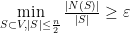$\varepsilon$ -vertex-expander if $\min\limits_{ S\subset V, |S| \leq \frac{n}{2} } \frac{|N(S)|}{|S|} \geq \varepsilon$ .

Remark 3: The reason for the restriction $|S| \leq n/2$ is that we are examining the relative size of every cut in the graph, i.e., the number of edges crossing between $S$ and $V \setminus S$ , and we examine each case only once.

Problem 1: Show that the complete graph $K_{n}$ is

at least a $1/2$ -edge-expander.
a $1$ -vertex-expander. (We only consider $\varepsilon \in [0, 1]$ here.)

From the definition above, the maximum $\varepsilon$ , which makes $G = (V, E)$ an $\varepsilon$ -edge-expander, is an important criteria, leading to the definition of Cheeger constant.

Definition 4(Cheeger Constant): The Edge Expansion Ratio, or Cheeger constant, of graph $G = (V, E)$ with $|V| = n$ , denoted by $h(G)$ , is defined as

$h(G) = \min\limits_{S\subset V, |S| \leq \frac{n}{2}}\frac{|\partial S|}{|E(S, V)|}$

Remark 5: Actually, Cheeger constant can be defined alternatively as 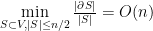$\min\limits_{S\subset V, |S| \leq n/2}\frac{|\partial S|}{|S|} = O(n)$ . We didn’t follow this definition since we want to keep $\varepsilon\in [0, 1]$ .

17.1.2. Spectral Expansion

To simplify our discussion, we focus on regular graphs in the rest of this lecture. Let $A = A(G)\in \mathbb{R}^{n \times n}$ denote the adjacency Matrix of a $d$ -regular graph $G = (V, E)$ with $|V| = n$ and $A$ being real symmetric, then $A$ has $n$ real eigenvalues, denoted by $\lambda_{1} \geq \lambda_{2} \geq \cdots \geq \lambda_n$ , and corresponding orthonormal eigenvectors $v_1, \dots, v_n$ with $A v_i = \lambda_i v_i$ . The spectrum of $A$ encodes a lot of information about the graph structure. Recall the following properties, which we have seen in previous lectures.

The largest eigenvalue is $\lambda_1 = d$ and the corresponding eigenvector is $v_1 = (1/\sqrt{n}, \dots, 1/\sqrt{n})$ .
The graph $G$ is connected if and only if $\lambda_1 > \lambda_2$ .
The graph is bipartite if and only if $\lambda_1 = -\lambda_n$ .

The definition of spectral expansion and spectral gap then follows.

Definition 6(Spectral Expansion): A graph $G = (V, E)$ with $|V| = n$ is a $\lambda$ -spectral-expander if $\lambda(G):= \max \{ |\lambda_2|, |\lambda_n| \} \leq \lambda$ .

In other words, the second largest eigenvalue of $A(G)$ , in absolute value, is at most $\lambda$ . This also gives rise to the definition of Ramanujan graph.

Definition 7(Ramanujan graph): A connected $d$ -regular graph $G$ is a Ramanujan graph if 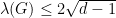$\lambda (G)\leq 2\sqrt{d-1}$ .

We now refer to the spectral gap.

Definition 8(Spectral Gap): The spectral gap of $d$ -regular graph $G$ is $\lambda_{1} - \lambda(G)$ .

Remark 9: Sometimes the spectral gap is defined as $\lambda_1 - \lambda_2$ , which is often referred as one-sided.

Problem 2:

Show that the complete graph $K_{n}$ has spectral gap $n - 2$ . Actually, we can also show that the one-sided spectral gap is $n$ .
Show that the complete bipartite graph $K_{m, n}$ has spectral gap $0$ . (Hint: use the spectral property above.)

17.2. Relating Two Definitions

It is not so obvious that the combinatorial and spectral versions of expansion are related. In this section, we will introduce two relations between edge and spectral expansion: the Expander-Mixing Lemma and Cheeger’s inequality.

17.2.1. The Expander-Mixing Lemma

Lemma 10(Expander-Mixing Lemma[2]): Let $G = (V, E)$ be a $d$ -regular graph with $n$ vertices and eigenvalues $\lambda_1 \geq \dots \geq \lambda_n$ . Then for all $S, T \subset V$ :

$\Bigg| |E(S, T)| - \frac{d|S|\cdot |T|}{n}\Bigg| \leq \lambda(G) \sqrt{|S|\cdot |T|}.$

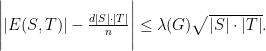
As we can see, the left-hand side measures the deviation between two quantities:

$|E(S, T)|$ : the number of edges between the two subsets $S$ and $T$ .
$|S|\cdot |T|\cdot d/n$ : the expected number of edges between two subsets $S$ and $T$ , drawn from an Erdos–Renyi random graph $G(n, d/n)$ .

The Expander-Mixing lemma tell us a small $\lambda(G)$ (a.k.a. large spectral gap) implies that this discrepancy is small, leading to the fact that the graph is nearly random in this sense, as discussed in [1]. We should mention that the converse of expander-mixing is true as well, stated as follows.

Lemma 11(Expander-Mixing Lemma Converse [4]): Let $G = (V, E)$ be a $d$ -regular graph with $n$ vertices and eigenvalues $\lambda_1 \geq \dots \geq \lambda_n$ satisfying:

$\Bigg| |E(S, T)| - \frac{d|S|\cdot |T|}{n}\Bigg| \leq \rho \sqrt{|S|\cdot |T|}.$

for any two disjoint subsets $S,T\subset V$ and some positive $\rho$ . Then $\lambda(G) \leq O(\rho \cdot(1 + \log(d/\rho)))$ .

Proof of Expander-Mixing Lemma: Recall that the adjacency matrix $A$ has eigenvalues $\lambda_1 \geq \dots \geq \lambda_n$ with corresponding orthonormal eigenvectors $v_1, \dots, v_n$ . Let $1_S$ and $1_T$ be the characteristic vectors of subsets $S$ and $T$ (a.k.a., the $v$ -th coordinate of $1_S$ is $1$ if $v\in S$ and $0$ otherwise). We then decompose $1_S$ and $1_T$ in the orthonormal basis of eigenvectors $v_1, \dots, v_n$ as

$1_S = \sum\limits_{i=1}^n \alpha_i v_i, \quad 1_S = \sum\limits_{j=1}^n\beta_j v_j$ .

Observing that $|E(S, T)| = (1_S)^T A 1_T$ , we expand out the right hand side and apply orthogonality, which yields

$(1_S)^T A 1_T = \left (\sum\limits_{i=1}^n \alpha_i v_i \right)^T A \left (\sum\limits_{j=1}^n\beta_j v_j \right) = \sum\limits_{i=1}^n \lambda_i\alpha_i\beta_i = d\frac{|S|\cdot|T|}{n} + \sum\limits_{i=2}^n \lambda_i\alpha_i\beta_i$ .

where the last step follows from the facts $\lambda_1 = d$ with corresponding $v_1 = (1/\sqrt{n},\dots, 1/\sqrt{n})$ , $\alpha_1 =<1_S, v_1> = |S|/\sqrt{n}$ and $\beta_1 =<1_T, v_1> = |T|/\sqrt{n}$ . Shifting the first term on right hand side to the left, the desired result follows from Cauchy-Schwarz inequality:

$\left| |E(S, T)| - d\frac{|S||T|}{n} \right | = \left|\sum\limits_{i=2}^n\lambda_i\alpha_i\beta_i\right| \leq \lambda(G) \sum\limits_{i=2}^n |\alpha_i \beta_i| \leq \lambda(G) ||\alpha||_2 ||\beta ||_2 = \lambda(G) ||1_S||_2 ||1_T||_2 = \lambda(G)\sqrt{|S||T|}.$

Remark 12: If we normalize the adjacency matrix $A = A(G)$ and obtain $\bar{A} = (1/d) A$ , where each entry of $A$ is divided by $d$ , then the corresponding eigenvalues of $\bar{A}$ , namely $\bar{\lambda}_{1}\geq \dots \geq \bar{\lambda}_n$ , lie in the interval $[-1, 1]$ . The Expander-Mixing Lemma is in the form of

$\Bigg| |E(S, T)| - \frac{d|S|\cdot |T|}{n}\Bigg| \leq \bar{\lambda}(G)d \sqrt{|S|\cdot |T|}.$

It is sometimes convenient to consider the normalized spectrum. For example in random graph theory, it would be convenient to look at the normalized spectrum when the expected degree $d = O(\log n)$ . However, we can focus on the spectrum of $\latex A = A(G)$ without normalization when the expected degree $\latex d = O(1)$.

Regular $\lambda$ -spectral expanders with small $\lambda(G)$ (a.k.a. large spectral gap) have some of significant properties, listed as follows.

Corollary 13: An independent set , in a graph $G = (V, E)$ with $|V| = n$ , is a set of vertices $S$ , where no two vertices in $S$ are adjacent, i.e. with $|E(S, S)| = 0$ . An independent set $S$ , in a $d$ -regular $\alpha$ -spectral expander $G$ , has cardinality at most $\alpha n$ , i.e., $|S|\leq \alpha n$ , which follows immediately from Lemma 10(Expander-Mixing Lemma[2]).

Corollary 14: Given a graph $G = (V, E)$ with $|V| = n$ , the diameter of $G$ is defined as $\mathrm{diam}(G) = \max\limits_{u, v}d_{G}(u, v)$ , where $d_{G}(u, v)$ is the length of shortest path between $u$ and $v$ . If $G$ is a $d$ -regular $\alpha$ -spectral expander $G$ with $\alpha < d/2$ , then we have

$\Omega \Big( \frac{\log n}{\log d} \Big) \leq \mathrm{diam}(G) \leq O(\log n).$

17.2.2. Cheeger’s Inequality

As we have seen from previous discussion, spectral expansion implies strong structural properties on the edge-structure of graphs. In this section, we introduce another famous result, Cheeger’s inequality, indicating that the Cheeger constant(Edge Expansion Ratio) of a graph $G$ can be approximated by the its spectral gap $\lambda_1 - \lambda(G)$ .[6]

Theorem 15(Cheeger’s inequality, [3]): Let $G = (V, E)$ be a $d$ -regular graph with eigenvalues $\lambda_1\geq \cdots \geq \lambda_n$ , then

$\frac{d - \lambda_2}{2} \leq \min\limits_{S\subset V, |S|\leq n/2} \frac{|\partial S|}{|S|} \leq \sqrt{2d(d - \lambda_2)}$ .

In the normalized scenario $\bar{A} = (1/d)A(G)$ with eigenvalues $\bar{\lambda}_{1}, \cdots, \bar{\lambda}_n \in [-1, 1]$ , we have

$\frac{1 - \bar{\lambda}_2}{2} \leq h(G):=\min\limits_{S\subset V, |S|\leq n/2} \frac{|\partial S|}{|E(S, V)|} \leq \sqrt{2(1 - \bar{\lambda}_2)}$ .

Remark 16: The proof for the normalized scenario is different from the regular scenario. We should start from the desired quantity and finish the calculation step by step. However, the strategy are the same. We use the Rayleigh Quotient to obtain upper bound and lower bound.

In the context of $n\gg d$ , the estimate of spectral gap was given by Nilli Alon.

Theorem 17([5]): For every $d$ -regular graph $G$ , we have

$\lambda(G) \geq 2\sqrt{d - 1} - o_{n}(1)$

The $o_{n}(1)$ term is a quantity that tends to zero for every fixed $d$ as $n \to \infty$ .

[1]. Shlomo Horry, N. L. and Wigderson, A. (2006). Expander graphs andtheir applications.BULLETIN (New Series) OF THE AMERICAN MATHEMATICAL SOCIETY, 43(4).
[2]. Alon, N. and Chung, F. R. K. (1988). Explicit construction of linear sized tolerantnetworks.Discrete Mathematics, 42
[3]. Cheeger, J. (1970). A lower bound for the smallest eigenvalue of the laplacian.Problems inanalysis, 26.[Nilli, 1991] Nilli, A. (1991). On the secon
[4]. Yonatan Bilu, N. L. (2006). Lifts, discrepancy and nearly optimal spectral gap.Com-binatorica, 26
[5]. Nilli, A. (1991). On the second eigenvalue of a graph.Discrete Mathematics, 91(2):207–210.
[6]. Lovett, S. (2021). Lecture notes for expander graphs and high-dimensional expanders.