Lecture 15 – Spectral Theory of Hypergraphs

Definition 1. A hypergraph $\Gamma$ is a pair $\Gamma = (V,E)$ where $V$ is a finite set and $E\subset 2^V$ is a nonempty collection of subsets of $V$ . $\Gamma$ is called $k$ -uniform if
$E\subset{V\choose k}:=\{X\subset V:|X| = k\}$ . $\Gamma$ is called a graph if it is 2-uniform.

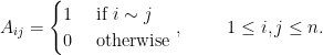
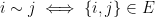
Our goal for this lecture is to explore the rudiments of the spectral theory of $k$ -uniform hypergraphs. The natural starting point, if only for inspiration, is the case of graphs. Letting $\Gamma = (V,E)$ be a graph, and identifying $V = \{1,2,\dotsc,n\}$ , we can begin by writing down the adjacency matrix $A = (A_{ij})$ of $\Gamma$ defined by

$A_{ij}=\begin{cases} 1&\text{ if }i\sim j\\ 0&\text{ otherwise} \end{cases}, \hspace{1cm}1\leq i,j\leq n.$

where $i\sim j\iff \{i,j\}\in E$ . In this case $i,j$ are said to be adjacent.

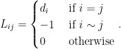
The spectral theory of $A$ is rich. For example, it made an appearance in our 202C class for the special case where $\Gamma$ is the Cayley graph of a group. Our main focus however will be the matrix $L = (L_{ij})$ , defined by

$L_{ij}=\begin{cases} d_{i}&\text{ if }i=j\\ -1&\text{ if }i\sim j\\ 0&\text{ otherwise} \end{cases}.$

where the degree $d_i$ is the number of edges containing $i\in V$ . If $D$ is the diagonal matrix of degrees, then we may also write $L = D-A$ . This matrix $L$ is called the Laplacian or Kirchoff matrix of $\Gamma$ . The terminology arises from the fact that as an operator on $\mathbb{C}^V$ , $L$ displays various properties canonically associated with the Laplacian on $\mathbb{R}^n$ ; e.g., mean value property, maximum principle, etc.. A very interesting paper of Wardetsky, Mathur, Kälberer, and Grinspun[6] explores these connections in detail, but they are outside of the scope of this lecture.

A few facts are worth collecting here- first, $L$ is a symmetric, positive semidefinite matrix in $M_n$ and hence admits nonnegative eigenvalues $0=\lambda_0\leq\lambda_1\leq\cdots\leq\lambda_{n-1}$ . $L$ always has zero as an eigenvalue, for example, via the vector $\mathbf{1} = (1,\dotsc,1)^T$ . But the multiplicity of said eigenvalue could be higher, depending on the number of connected components (Exercise 1). However when we assume $\Gamma$ is connected (i.e. contains a single connected component), it follows that $\lambda_1>0$ . In much of the literature, we are often interested in the interplay and connections between geometric and combinatorial properties of $\Gamma$ – things like its size, connectedness, density, or sparseness, for example; and the first eigenvalue $\lambda_1$ (either of $L$ or one of its many variants). For example…

Exercise 1.
(a) Show that the geometric multiplicity of the null eigenvalue of $L$ is the number of connected components of $\Gamma$ .
(b) Show $\lambda_1\leq n,$ with equality if and only if $\Gamma$ is the complete graph. Hint: if $\Gamma$ is not complete, relate its Laplacian and that of its “complement” (suitably defined) to the Laplacian of the complete graph, and use eigenvalue interlacing.

For a more detailed introduction to spectral graph theory, see Fan Chung’s book[1, Ch. 1].

Our next goal is to try and take these notions and structures and construct extensions, or analogues, for the case where $\Gamma$ is a $k$ -uniform hypergraph. As we shall see, this is not so easy. Consider if you desire the following perspective from simplicial homology (those unfamiliar or otherwise uninterested, skip to Definition 2).

One approach would be to try and construct $L$ not as a specific matrix, but as a descendant of an invariant of the topology of the underlying graph; which we could then hope admits a generalization to the case where the graph is instead a hypergraph. Specifically, the idea is to look at the homology of $\Gamma$ and build a Laplacian from its boundary operator- as follows.

Let $\Gamma$ be a graph and enumerate $E = \{e_1,\dotsc,e_m\}$ . To each unordered pair $e_j=\{v,w\}\in E$ pick an orientation $(v,w)$ or $(w,v)$ and let $\widetilde{E}$ be the set of all such oriented edges. Let $S = (S_{v,e}) \in M_{n\times m}$ be the matrix whose rows are indexed by $v\in V$ and whose columns are indexed by the ordered edges $e\in\widetilde{E}$ , defined by

$S_{v,e} = \begin{cases} 1&\text{if }e = (v,\cdot)\\ -1&\text{ if }e=(\cdot,v)\\ 0&\text{ otherwise} \end{cases}.$

It is left as an (unassigned) exercise to verify that $L=SS^T$ ; and in fact that the choice of orientations/signs in the preceding setup is completely arbitrary. Thinking of $S$ as a homomorphism mapping elements of the module $\mathbb{Z} E$ to the module $\mathbb{Z} V$ by matrix multiplication, we recognize $S$ as the boundary operator that is related to the homology groups of $\Gamma$ as a simplicial complex (see [3, Section 2.1, page 105]) and thus we have constructed $L$ as an invariant of the topology of $\Gamma$ (up to choices in the orientations of the edges).

But as it turns out, the capricious choice of orientation we made earlier to define $S$ is what makes graphs special. As soon as we allow 3-edges, or 1-edges for that matter, it is not at all obvious how to “orient” them, or how to distinguish between orientations (compare to the natural symbolic relationship $(v,w)=-(w,v)$ ). This, in fact, is a critically important distinction between graphs and hypergraphs. The answer is that we need more than linear operators, and so we look to tensors. The exposition that follows roughly follows two papers of Qi[4,5].

Definition 2. A tensor $\mathcal{T}$ of order $m$ and dimension $n$ over a field $\mathbb{F}$ is a multidimensional array

$\mathcal{T} = (t_{i_1i_2\cdots i_m}),\hspace{1cm}1\leq i_1,\dotsc,i_m\leq n.$

where each entry $t_{i_1i_1\cdots i_m}\in\mathbb{F}$ . We call $\cal{T}$ an $(m,n)$ -tensor over $\mathbb{F}$ .

We can think of an $(m,n)$ -tensor as a hypercubic array of size $n\times n\times\cdots\times n$ , $m$ times). All of the tensors presented here are understood to be over $\mathbb{C}$ . The case $(2,n)$ recovers the usual $n\times n$ square matrices. If $x\in\mathbb{C}^n$ then we define the product $\mathcal{T}x^{m-1}\in\mathbb{C}^n$ by

$(\mathcal{T}x^{m-1})_i = \sum_{i_2,\dotsc,i_m=1}^n t_{ii_2\cdots i_m}x_{i_2}\cdots x_{i_m},\hspace{1cm}1\leq i\leq n.$

(The expression $\mathcal{T}x^{m-1}\in\mathbb{C}^n$ is conventional notation.) Also as a matter of notation, for $x\in \mathbb{C}^n$ and $k\geq 0$ , let $x^{[k]}\in\mathbb{C}^n$ be given by $(x^{[k]})_i = x_i^k$ . There are lots of analogous notions and properties for tensors as compared to usual matrices; for example, we have the following formulation of the spectrum of a tensor.

Definition 3. Let $\cal{T}$ be an $(m,n)$ -tensor. Then we say $\lambda\in\mathbb{C}$ is an eigenvalue of $\cal{T}$ if there exists a nonzero vector $x\in\mathbb{C}^n$ , called an eigenvector of $\mathcal{T}$ , which satisfies $\mathcal{T} x^{m-1} = \lambda x^{[m-1]}.$

Notice that no $(k,n)$ tensor $\mathcal{T}$ for $k\geq 3$ defines a true linear operator on $\mathbb{C}^n$ , and hence we may not a priori speak of eigenspaces, kernels, etc. and their linear algebraic structure. (These notions do have meaning, but they require the tools of algebraic geometry to properly formulate, and are outside of our scope.) Nevertheless, we can construct tensors associated to $k$ -uniform hypergraphs that will give rise to various eigenvalues. And if so, can we find relationships between the geometry of a hypergraph and its eigenvalues?

Definition 4. Let $\Gamma=(V,E)$ be a $k$ -uniform hypergraph on $n$ vertices. The adjacency tensor of $\Gamma$ is the $(k,n)$ -tensor $\mathcal{A} = (a_{i_1\cdots i_k})$ defined as follows. For each edge $e = \{i_1,\dotsc,i_k\}\in E$ ,

$a_{i_1i_2\cdots i_k} = \frac{1}{(k-1)!},$

and likewise for any rearrangment $(i_1',\dotsc,i_k')$ of the vertices in $e$ . The values of $\mathcal{A}$ are defined to be zero otherwise. The degree tensor of $\Gamma$ is the $(k,n)$ -tensor $\mathcal{D}=(d_{i_1\cdots i_k})$ defined by

$d_{i\cdots i} = d_i,$

where $d_i$ is the number of edges containing $i$ , and the values of $\mathcal{D}$ are defined to be zero otherwise. The Laplacian tensor is the $(k,n)$ tensor $\mathcal{L}= (l_{i_1\cdots i_k})$ defined by $\mathcal{L} = \mathcal{D}-\mathcal{A}$ .

A brief remark- our choice to focus on $k$ -uniform hypergraphs is merely to simplify the exposition. There are well-developed versions of Definition 4 for general hypergraphs[2], but they are harder to write down and explore in this setting. With these fundamental notions established, the goal for the remainder will be to write down and explore a few basic propositions regarding the eigenvalues and eigenvectors of the tensors of a hypergraph $\Gamma$ .

Proposition 1. Let $\Gamma$ be a $k$ -uniform hypergraph, with $k\geq 3$ , on $n$ vertices and $\mathcal{L}$ its Laplacian tensor.

Let $\mathbf{e}_j\in\mathbb{C}^n$ denote the $j$ -th standard basis vector. Then $\mathbf{e}_j$ is an eigenvector of $\mathcal{L}$ with eigenvalue $d_j$ .
The vector $\mathbf{1}$ occurs as an eigenvector of $\mathcal{L}$ with eigenvalue 0.

Proof. This is an exercise in calculations with tensors. For the first claim let $1\leq j\leq n$ be fixed, and notice that for any $m\geq 1$ , $\mathbf{e}_j^{[m]} = \mathbf{e}_j$ and hence for each $1\leq i\leq n$ , it holds

Notice that $a_{i_1\cdots i_k} = 0$ if any of the $i_k$ ‘s are repeated, and that $d_{ij\cdots j} = d_i$ if $i=j$ and 0 otherwise. It follows that $\mathcal{L}\mathbf{e}_j^{k-1} = d_j\mathbf{e}_j^{[k-1]}$ . For the second claim, again we have $\mathbf{1}^{[m]} = \mathbf{1}$ for any $m$ , and hence

where, with some abuse of notation in the second line, we emphasize that the sum contains all permutations of the $k-1$ terminal points in each edge $e=\{i,i_2,\dotsc,i_k\}\in E$ . -QED.

Exercise 2. Let $\Gamma$ be a $k$ -uniform hypergraph and $\mathcal{A}$ its adjacency tensor. Show that $\mathbf{e}_j$ occurs as an eigenvector of $\mathcal{A}$ with eigenvalue 0 for each $j$ . Sanity check: why does this not imply that $\mathcal{A}=0$ ?

Our next proposition is a statement about the distribution of eigenvalues.

Proposition 2. Let $\Gamma$ be a $k$ -uniform hypergraph on $n$ vertices, and $\mathcal{L}$ its Laplacian tensor. Let $\Delta$ denote the maximum degree of $\Gamma$ . Then all of the eigenvalues of $\mathcal{L}$ lie in the disk $\{\lambda\in\mathbb{C}:|\lambda-\Delta|\leq\Delta\}$ .

Proof. ([4, Thm. 6]) Let $\lambda\in\mathbb{C}$ be an eigenvalue for $\mathcal{L}$ , and let $x\in\mathbb{C}^n$ be a corresponding eigenvector. Assume we have

$|x_i| = \max_{j=1,\dotsc,n}|x_j| \neq 0.$

Then by definition, it holds $\mathcal{L}x^{m-1} = \lambda x^{[m-1]}$ , which in the $i$ -th component reads

$\lambda x_i^{k-1} = \sum_{i_2,\dotsc,i_k=1}^n l_{i,i_2,\dotsc, i_k} x_{i_2}\cdots x_{i_k}.$

Removing a single term from the right-hand side, we get

But from the definition of $\mathcal{L}$ we recognize $l_{i\cdots i}$ as $d_i$ and hence by choice of $i$ , we can estimate

where in the final equality we are using the definition of $\mathcal{L}$ and are recalling the calculation in the proof of proposition 1. We have hence proved that all eigenvalues $\lambda$ lie in a closed disk centered on $d_i\in\mathbb{C}$ of the same radius; but this $i\in V$ depends on the unknown eigenvector $x\in\mathbb{C}^n$ , so by observing that for any $j\in V$ ,

$\{\lambda\in\mathbb{C}:|\lambda-d_j|\leq d_j\}\subset \{\lambda\in\mathbb{C}:|\lambda-\Delta|\leq\Delta\}$

the claim follows. -QED

Exercise 3. Let $\Gamma$ be a $k$ -uniform hypergraph on $n$ vertices and $\mathcal{A}$ its adjacency tensor. Show that all of the eigenvalues of $\mathcal{A}$ lie in the disk $\{\lambda\in\mathbb{C}:|\lambda|\leq\Delta\}$ .

For our final proposition, we strive for an analogue of Exercise 1(a)- that is, a relationship between the “size of the kernel” and the connected components of $\Gamma$ . However for $k$ -uniform hypergraphs, $\mathcal{L}$ will not be a linear operator for any $k\geq 3$ , and hence a kernel is not well-defined a priori. But as we saw in Proposition 1, the same vector $\mathbf{1}$ shows up as an eigenvector for the null eigenvalue, and hence we are suspicious that more can be said.

A few small preliminaries are in order. A vector $x\in\mathbb{C}^n$ is called a binary vector if each of its components $x_i$ are either 0 or 1 for $1\leq i\leq n$ . The support of a vector $x\in\mathbb{C}^n$ is the set $\text{supp}(x) = \{1\leq i\leq n:x_i\neq 0\}$ . If $\mathcal{T}$ is a $(k,n)$ -tensor over $\mathbb{C}$ , then an an eigenvector $x\in\mathbb{C}^n$ associated to eigenvalue $\lambda\in\mathbb{C}$ is called a minimal binary eigenvector associated to $\lambda$ if $x$ is a binary vector, and if there does not exist another binary eigenvector $y\in\mathbb{C}^n$ with eigenvalue $\lambda$ for which $\text{supp}(y)$ is a proper subset of $\text{supp}(x)$ .

Proposition 3. Let $\Gamma$ be a $k$ -uniform hypergraph on $n$ vertices with Laplacian tensor $\mathcal{L}$ . A binary vector $x\in\mathbb{C}^n$ is a minimal binary eigenvector associated to $\lambda = 0$ if and only if $\text{supp}(x)$ is the vertex set of a connected component of $\Gamma$

Proof. We first observe using the proof of Proposition 1 that a nonzero vector $x\in\mathbb{C}^n$ is an eigenvector associated to $\lambda=0$ if and only if, for each $1\leq i\leq n$ , it holds

( $\implies$ ). Let $x\in\mathbb{C}^n$ be any minimal binary eigenvector associated to $\lambda=0$ and let $i\in\text{supp}(x)$ . It follows from equation (1) that for any $(i,i_2,\dotsc,i_k)\in E$ it holds $i_2,\dotsc,i_k\in \text{supp}(x)$ (otherwise, there will not be enough terms in the sum to achieve $d_i$ ). Applying this observation inductively to adjacent vertices in $\text{supp}(x)$ , we see that the vertices $i\in\text{supp}(x)$ form either the vertex set of one component of $\Gamma$ , or the disjoint union of several. But the latter case is incompatible with minimality, since any binary vector supported on a single component will give rise to an eigenvector with eigenvalue $\lambda=0$ (check!).

( $\impliedby$ ). Now assume simply that $x\in\mathbb{C}^n$ is a binary vector with support equal to a single connected component of $\Gamma$ . A short calculation verifies that the components $x_i$ for $i\in\text{supp}(x)$ satisfy equation (1), and hence that $x$ is a binary eigenvector for $\mathcal{L}$ assosicated to eigenvalue $\lambda=0$ . All that remains to be checked is that $x$ is minimal; to this end, suppose $y\in\mathbb{C}^n$ is another binary eigenvector, and that $\text{supp}(y)\subsetneq \text{supp}(x)$ . Then there must exist some vertex $i\in\text{supp}(y)$ for which there exists some edge $e= \{i,i_2,\dots,i_k\}\in E$ and an index $j\in e$ which does not belong to $\text{supp}(y)$ . But then,

and equation (1) cannot hold for $y$ , a contradiction. -QED

Corollary 1. A $k$ -uniform hypergraph $\Gamma$ is connected if and only if the vector $\mathbf{1}$ is the unique minimal binary eigenvector with eigenvalue $\lambda=0$ .

References and Further Reading.

Fan Chung. Spectral Graph Theory. 1997.
Cunxiang Duan, Ligong Wang, Xihe Li, et al. Some properties of the signless laplacian andnormalized laplacian tensors of general hypergraphs. Taiwanese Journal of Mathematics, 24(2). 2020.
Allen Hatcher. Algebraic topology. 2005.
Liqun Qi. Eigenvalues of a real supersymmetric tensor. Journal of Symbolic Computation, 40(6). 2005.
Liqun Qi. H+-eigenvalues of laplacian and signless laplacian tensors. Communications in Mathematical Sciences, 12(6). 2013.
Max Wardetzky, Saurabh Mathur, Felix Kälberer, and Eitan Grinspun. Discrete laplace operators: no free lunch. In Symposium on Geometry processing. 2007.

Lecture 15 – Spectral Theory of Hypergraphs

Like this:

Published by s5robert

Leave a ReplyCancel reply

Share this:

Like this:

Published by s5robert

Leave a ReplyCancel reply